1. Introduction to Examples
This section demonstrates the core functionality of the indeterminatebeam package with examples. Examples 5, 6, 7 and 8 have been taken from the Hibbeler textbook [2].
You can follow along with examples online: ![]()
![]()
In order to effectively use the package online you should first run the cell that initialises the notebook by installing the package.
# RUN THIS CELL FIRST TO INITIALISE GOOGLE NOTEBOOK!!!!
!pip install indeterminatebeam
%matplotlib inline

# import beam and supports
from indeterminatebeam import Beam, Support

# import loads (all load types imported for reference)
from indeterminatebeam import (
    PointTorque,
    PointLoad,
    PointLoadV,
    PointLoadH,
    UDL,
    UDLV,
    UDLH,
    TrapezoidalLoad,
    TrapezoidalLoadV,
    TrapezoidalLoadH,
    DistributedLoad,
    DistributedLoadV,
    DistributedLoadH
)

# Note: load ending in V are vertical loads
# load ending in H are horizontal loads
# load not ending in either takes angle as an input (except torque)
You can also approach the problems using the web-based graphical user interface

2. Basic Usage (Readme example)
2.1 Basic Usage
Specifications
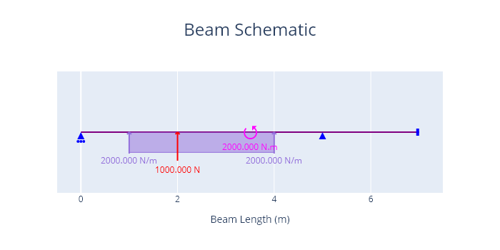
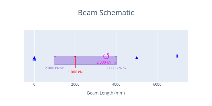
A diagram of the problem is shown below.
Results
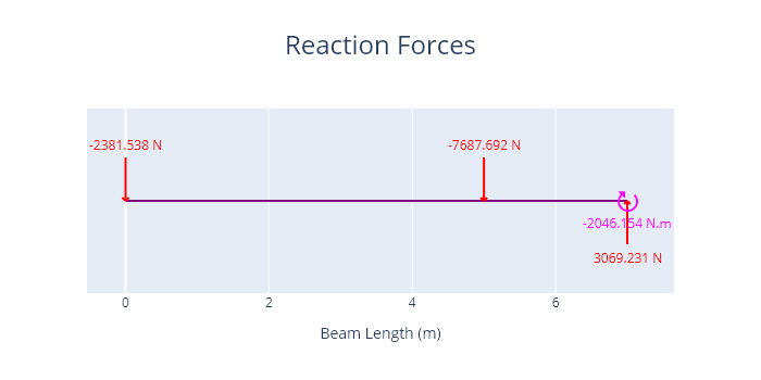
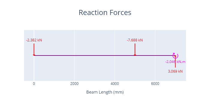
A plot of the reactions is shown below.
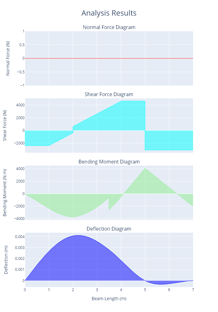
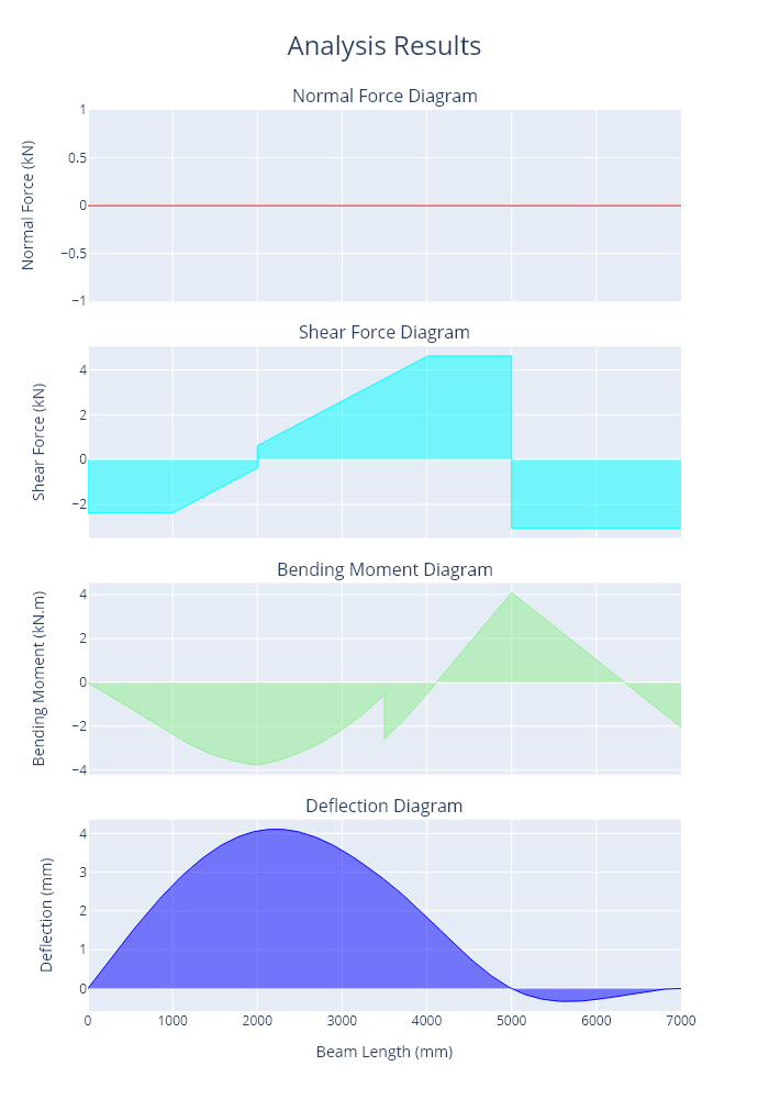
A plot of the axial force, shear force, bending moments and deflections is shown below.
Code
# Arbritrary example defined in README.md
from indeterminatebeam import Beam, Support, PointLoadV, PointTorque, UDLV, DistributedLoadV
beam = Beam(7)                          # Initialize a Beam object of length 7 m with E and I as defaults
beam_2 = Beam(9,E=2000, I =100000)      # Initialize a Beam specifying some beam parameters

a = Support(5,(1,1,0))                  # Defines a pin support at location x = 5 m
b = Support(0,(0,1,0))                  # Defines a roller support at location x = 0 m
c = Support(7,(1,1,1))                  # Defines a fixed support at location x = 7 m
beam.add_supports(a,b,c)

load_1 = PointLoadV(1000,2)                # Defines a point load of 1000 N acting up, at location x = 2 m
load_2 = DistributedLoadV(2000,(1,4))      # Defines a 2000 N/m UDL from location x = 1 m to x = 4 m
load_3 = PointTorque(2*10**3, 3.5)            # Defines a 2*10**3 N.m point torque at location x = 3.5 m
beam.add_loads(load_1,load_2,load_3)    # Assign the support objects to a beam object created earlier

beam.analyse()

fig_1 = beam.plot_beam_external()
fig_1.show()

fig_2 = beam.plot_beam_internal()
fig_2.show()

# save the results (optional)
# Can save figure using ``fig.write_image("./results.pdf")`` (can change extension to be
# png, jpg, svg or other formats as reired). Requires pip install -U kaleido

# fig_1.write_image("./readme_example_diagram.png")
# fig_2.write_image("./readme_example_internal.png")
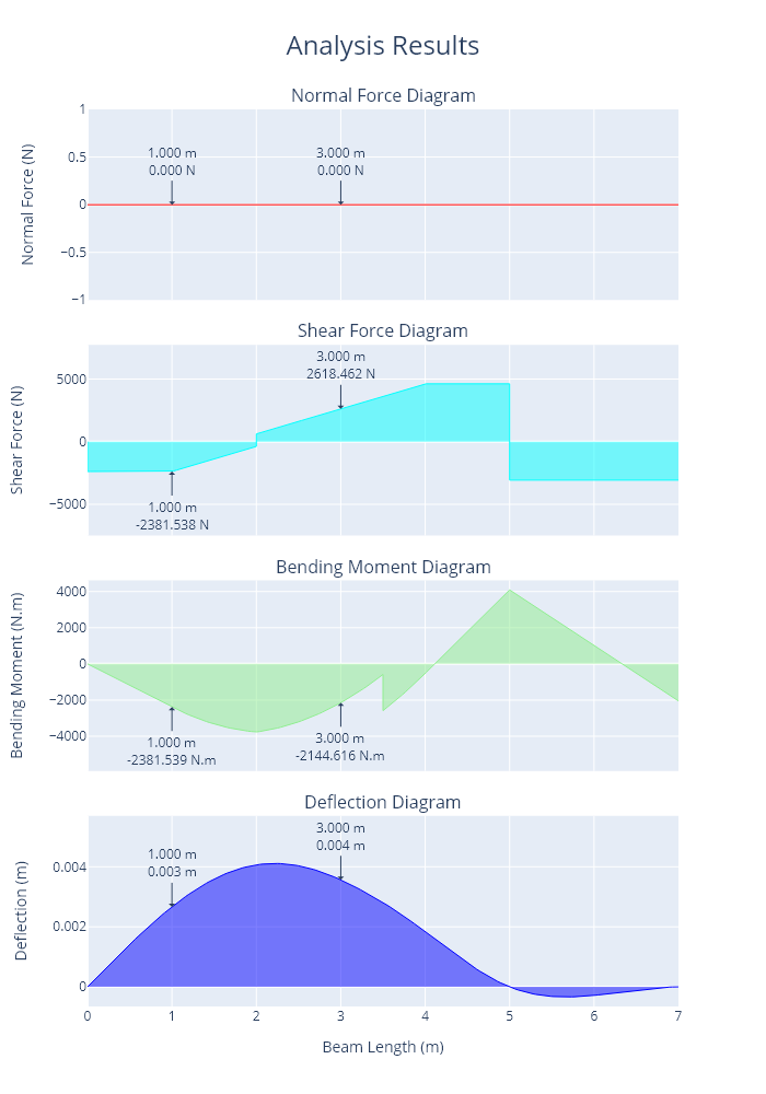
2.2 Querying Data
Specifications
The same beam as presented in 2(a) is analysed further for specific information. Querys are set at specific coordinates to allow for more precise data, rather than a general graph over view.
Results
The program outputs the following text.:
bending moments at 3 m: -2144.6156464615
shear forces at 1,2,3,4,5m points: [-2381.5384615385, 618.4617384615, 2618.4617384615, 4618.4615384615, 4618.4615384615]
normal force absolute max: 0.0
deflection max: 0.0041098881
A plot of the axial force, shear force, bending moments and deflections is shown below.
Code
# Run section 2a (prior to running this example)

# query for the data at a specfic point (note units are not provided)
print("bending moments at 3 m: " + str(beam.get_bending_moment(3)))
print("shear forces at 1,2,3,4,5m points: " + str(beam.get_shear_force(1,2,3,4,5)))
print("normal force absolute max: " + str(beam.get_normal_force(return_absmax=True)))
print("deflection max: " + str(beam.get_deflection(return_max = True)))

##add a query point to a plot (adds values on plot)
beam.add_query_points(1,3,5)
beam.remove_query_points(5)

## plot the results for the beam
fig = beam.plot_beam_internal()
fig.show()
2.3 Specifing units
Specifications
The same beam as presented in 2(a) is set up using alternative units for the same result. Note that units are used to modify both inputs and outputs. Default units are SI (N and m).
A diagram of the problem is shown below.
Results
A plot of the reactions is shown below.
A plot of the axial force, shear force, bending moments and deflections is shown below.
Code
# Readme example as a demonstration for changing units
# used and presented in following example. Note that
# the example is conceptually identical only with
# different units.

# update units usings the update_units() function.
# use the command below for more information.
# help(beam.update_units)

# note: initialising beam with the anticipation that units will be updated
beam = Beam(7000, E = 200 * 10 **6, I = 9.05 * 10 **6)

beam.update_units(key='length', unit='mm')
beam.update_units('force', 'kN')
beam.update_units('distributed', 'kN/m')
beam.update_units('moment', 'kN.m')
beam.update_units('E', 'kPa')
beam.update_units('I', 'mm4')
beam.update_units('deflection', 'mm')

a = Support(5000,(1,1,0))               # Defines a pin support at location x = 5 m (x = 5000 mm)
b = Support(0,(0,1,0))                  # Defines a roller support at location x = 0 m
c = Support(7000,(1,1,1))               # Defines a fixed support at location x = 7 m (x = 7000 mm)
beam.add_supports(a,b,c)

load_1 = PointLoadV(1,2000)             # Defines a point load of 1000 N (1 kN) acting up, at location x = 2 m
load_2 = DistributedLoadV(2,(1000,4000))      # Defines a 2000 N/m (2 kN/m) UDL from location x = 1 m to x = 4 m
load_3 = PointTorque(2, 3500)           # Defines a 2*10**3 N.m (2 kN.m) point torque at location x = 3.5 m
beam.add_loads(load_1,load_2,load_3)    # Assign the support objects to a beam object created earlier

beam.analyse()
fig_1 = beam.plot_beam_external()
fig_1.show()

fig_2 = beam.plot_beam_internal()
fig_2.show()
2.4 Exporting Results
Specifications
The beam results from 2(a) can also be exported to a table via printing or by exporting to excel.
Results
x [m] |
Axial [N] |
Shear [N] |
Moment [N.m] |
Deflection [m] |
|---|---|---|---|---|
0.0 |
0 |
-2381.538 |
0.0 |
0.0 |
0.778 |
0 |
-2381.538 |
-1852.308 |
0.002 |
1.556 |
0 |
-1270.427 |
-3395.973 |
0.004 |
2.333 |
0 |
1285.128 |
-3445.812 |
0.004 |
3.111 |
0 |
2840.684 |
-1841.33 |
0.003 |
3.889 |
0 |
4396.239 |
-1026.971 |
0.002 |
4.667 |
0 |
4618.462 |
2552.821 |
0.0 |
5.444 |
0 |
-3069.231 |
2728.205 |
-0.0 |
6.222 |
0 |
-3069.231 |
341.026 |
-0.0 |
7.0 |
0 |
0.0 |
0.0 |
0.0 |
Code
# Arbritrary example defined in README.md
from indeterminatebeam import Beam, Support, PointLoadV, PointTorque, UDLV, DistributedLoadV
beam = Beam(7)                          # Initialize a Beam object of length 7 m with E and I as defaults
beam_2 = Beam(9,E=2000, I =100000)      # Initialize a Beam specifying some beam parameters

a = Support(5,(1,1,0))                  # Defines a pin support at location x = 5 m
b = Support(0,(0,1,0))                  # Defines a roller support at location x = 0 m
c = Support(7,(1,1,1))                  # Defines a fixed support at location x = 7 m
beam.add_supports(a,b,c)

load_1 = PointLoadV(1000,2)                # Defines a point load of 1000 N acting up, at location x = 2 m
load_2 = DistributedLoadV(2000,(1,4))      # Defines a 2000 N/m UDL from location x = 1 m to x = 4 m
load_3 = PointTorque(2*10**3, 3.5)            # Defines a 2*10**3 N.m point torque at location x = 3.5 m
beam.add_loads(load_1,load_2,load_3)    # Assign the support objects to a beam object created earlier

beam.analyse()

# print results as a table with 10 points
beam.print_results_table(num_points=10, max_dp=3)

# optionally export as a csv
# beam.export_results_csv(filename="filename.csv", num_points=100, max_dp=10)
3. Support class breakdown
Representation
Supports can be created for a range of degrees of freedom. In order to ensure all possible supports are visually distinct a seperate support represenation has been used for each different possible degree of freedom combination.
The creation of different supports is shown in the code and diagram below.
Code
# The parameters for a support class are as below, taken from the docstring
# for the Support class __init__ method.

# Parameters:
#         -----------
#         coord: float
#             x coordinate of support on a beam in m (default 0)
#         fixed: tuple of 3 booleans
#             Degrees of freedom that are fixed on a beam for movement in
#             x, y and bending, 1 represents fixed and 0 represents free
#             (default (1,1,1))
#         kx :
#             stiffness of x support (N/m), if set will overide the
#             value placed in the fixed tuple. (default = None)
#         ky : (positive number)
#             stiffness of y support (N/m), if set will overide the
#             value placed in the fixed tuple. (default = None)


# Lets define every possible degree of freedom combination for
# supports below, and view them on a plot:
support_0 = Support(0, (1,1,1))     # conventional fixed support
support_1 = Support(1, (1,1,0))     # conventional pin support
support_2 = Support(2, (1,0,1))
support_3 = Support(3, (0,1,1))
support_4 = Support(4, (0,0,1))
support_5 = Support(5, (0,1,0))     # conventional roller support
support_6 = Support(6, (1,0,0))

# Note we could also explicitly define parameters as follows:
support_0 = Support(coord=0, fixed=(1,1,1))

# Now lets define some spring supports
support_7 = Support(7, (0,0,0), kx = 10)    #spring in x direction only
support_8 = Support(8, (0,0,0), ky = 5)     # spring in y direction only
support_9 = Support(9, (0,0,0), kx = 100, ky = 100)     # spring in x and y direction

# Now lets define a support which is fixed in one degree of freedom
# but has a spring stiffness in another degree of freedom
support_10 = Support(10, (0,1,0), kx = 10) #spring in x direction, fixed in y direction
support_11 = Support(11, (0,1,1), kx = 10) #spring in x direction, fixed in y and m direction

# Note we could also do the following for the same result since the spring
# stiffness overides the fixed boolean in respective directions
support_10 = Support(10, (1,1,0), kx =10)

# Now lets plot all the supports we have created
beam = Beam(11)

beam.add_supports(
    support_0,
    support_1,
    support_2,
    support_3,
    support_4,
    support_5,
    support_6,
    support_7,
    support_8,
    support_9,
    support_10,
    support_11,
)

fig = beam.plot_beam_diagram()
fig.show()
4. Load classes breakdown
4.1 Point Torque
Representation
A beam loaded with point torques is shown below.
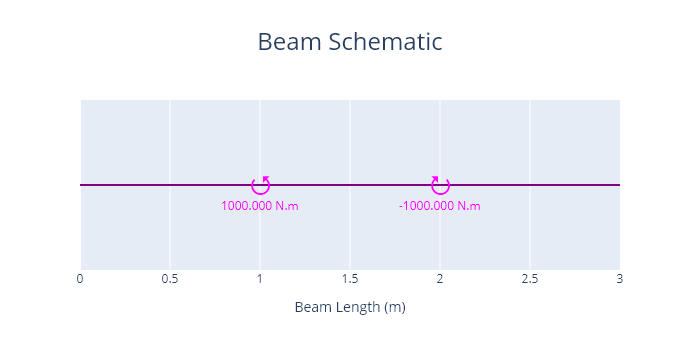
Code
# defined using a force (technically a moment, however force is used to maintain consistenct for all load classes) and a coordinate. An anti-clockwise moment is positive by convention of this package.
load_1 = PointTorque(force=1000, coord=1)
load_2 = PointTorque(force=-1000, coord=2)

# Plotting the loads
beam = Beam(3)
beam.add_loads(
    load_1,
    load_2
)

fig = beam.plot_beam_diagram()
fig.show()
4.2 Point Load
Representation
A beam loaded with point loads is shown below.
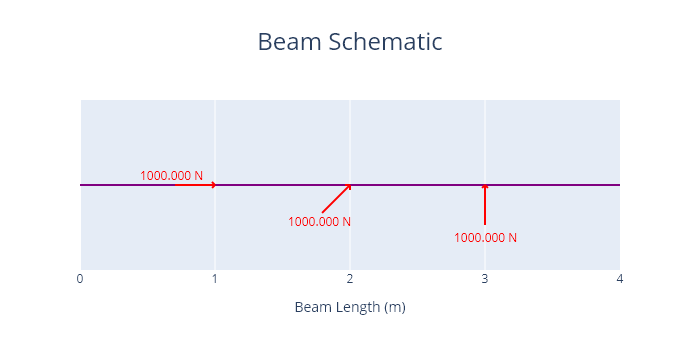
Code
# defined by force, coord and angle (0)
load_1 = PointLoad(force=1000, coord=1, angle=0)
load_2 = PointLoad(force=1000, coord=2, angle=45)
load_3 = PointLoad(force=1000, coord=3, angle=90)

# Plotting the loads
beam = Beam(4)
beam.add_loads(
    load_1,
    load_2,
    load_3
)

fig = beam.plot_beam_diagram()
fig.show()
4.3 Uniformly Distributed Load (UDL)
Representation
A beam loaded with uniformly distributed loads is shown below.
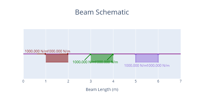
Code
# defined by force, span (tuple with start and end point)
# and angle of force
load_1 = UDL(force=1000, span=(1,2), angle = 0)
load_2 = UDL(force=1000, span=(3,4), angle = 45)
load_3 = UDL(force=1000, span=(5,6), angle = 90)

# Plotting the loads
beam = Beam(7)
beam.add_loads(
    load_1,
    load_2,
    load_3
)

fig = beam.plot_beam_diagram()
fig.show()
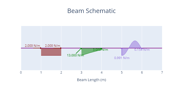
4.4 Trapezoidal Load
Representation
A beam loaded with trapezoidal loads is shown below.
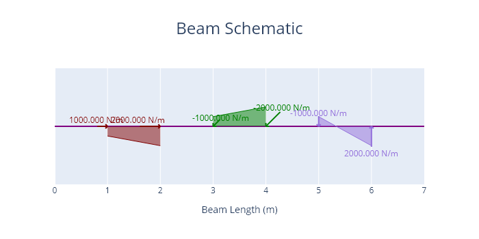
Code
# defined by force (tuple with start and end force),
# span (tuple with start and end point) and angle of force
load_1 = TrapezoidalLoad(force=(1000,2000), span=(1,2), angle = 0)
load_2 = TrapezoidalLoad(force=(-1000,-2000), span=(3,4), angle = 45)
load_3 = TrapezoidalLoad(force=(-1000,2000), span=(5,6), angle = 90)

# Plotting the loads
beam = Beam(7)
beam.add_loads(
    load_1,
    load_2,
    load_3
)

fig = beam.plot_beam_diagram()
fig.show()
4.5 Distributed Load
Representation
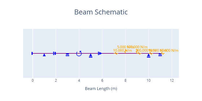
A beam loaded with distributed loads is shown below.
It should be noted that distributed loads are treated differently by the program as compared to all other load objects. Distributed loads are set up to be more flexible but at the cost of the calculations running much slower. Where other functions can be used the distributed load type object should be avoided.
Code
# defined with Sympy expression of the distributed load function
# expressed using variable x which represents the beam x-coordinate.
# Requires quotation marks around expression. As with the UDL and
# Trapezoidal load classes other parameters to express are the span
# (tuple with start and end point) and angle of force.
# NOTE: where UDL or Trapezoidal load classes can be specified (linear functions)
# they should be used for quicker analysis times.

load_1 = DistributedLoad(expr= "2", span=(1,2), angle = 0)
load_2 = DistributedLoad(expr= "2*(x-6)**2 -5", span=(3,4), angle = 45)
load_3 = DistributedLoad(expr= "cos(5*x)", span=(5,6), angle = 90)

# Plotting the loads
beam = Beam(7)
beam.add_loads(
    load_1,
    load_2,
    load_3
)

fig = beam.plot_beam_diagram()
fig.show()
4.6 Vertical and Horizontal load child classes
Representation
For all loads except the point torque an angle is specified for the direction of the load. If the load to be specified is to be completely vertical or completely horizontal a V (vertical) or a H (horizontal) can be added at the end of the class name, and the angle does then not need to be specified.
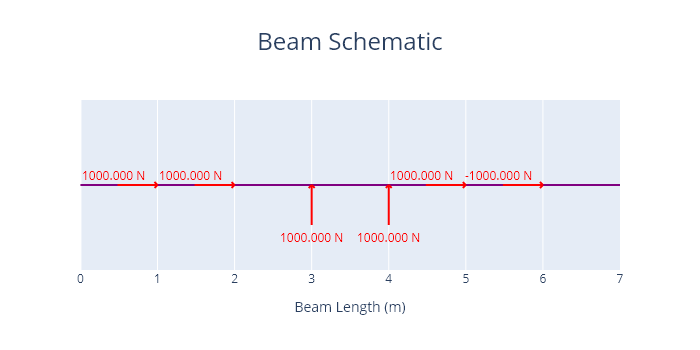
Code
# for all loads except the point torque an angle is specified for the
# direction of the load. If the load to be specified is to be completely
# vertical or completely horizontal a V (vertical) or a H (horizontal)
# can be added at the end of the class name, and the angle does then
# not need to be spefied.

# The following two loads are equivalent horizontal loads
load_1 = PointLoad(force=1000, coord=1, angle = 0)
load_2 = PointLoadH(force=1000, coord=2)

# The following two loads are equivalent vertical loads
load_3 = PointLoad(force=1000, coord=3, angle = 90)
load_4 = PointLoadV(force=1000, coord=4)

# The following two loads are also equivalent (a negative sign
# esentially changes the load direction by 180 degrees).
load_5 = PointLoad(force=1000, coord=5, angle = 0)
load_6 = PointLoad(force=-1000, coord=6, angle = 180)


# Plotting the loads
beam = Beam(7)
beam.add_loads(
    load_1,
    load_2,
    load_3,
    load_4,
    load_5,
    load_6
)

fig = beam.plot_beam_diagram()
fig.show()
5. Statically Determinate Beam
This example has been taken from Ex 12.14 in the Hibbeler textbook [2].
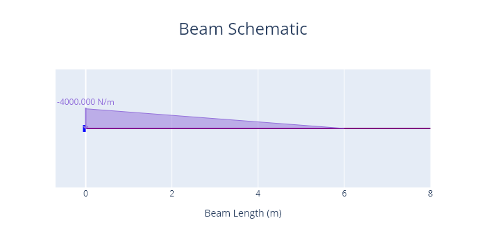
Specifications
An 8 m long cantilever AB is fixed at A (x = 0 m).
The beam is subject to a trapezoidal load of magnitude 4000 N/m acting downwards at x = 0 m, linearly decreasing in magnitude to a value of 0 N/m at x = 6 m.
Determine the displacement at B (x = 8 m) as a function of EI.
A diagram of the problem is shown below.
Results
The deflection is -244800.0036000013 (N.m3) / EI (N.m2)
Code
# Statically Determinate beam (Ex 12.14 Hibbeler)
# Determine the displacement at x = 8m for the following structure
# 8 m long fixed at A (x = 0m)
# A trapezoidal load of - 4000 N/m at x = 0 m descending to 0 N/m at x = 6 m.

beam = Beam(8, E=1, I = 1)     ##EI Defined to be 1 get the deflection as a function of EI

a = Support(0, (1,1,1))             ##explicitly stated although this is equivalent to Support() as the defaults are for a cantilever on the left of the beam.

load_1 = TrapezoidalLoadV((-4000,0),(0,6))

beam.add_supports(a)
beam.add_loads(load_1)

beam.analyse()
print(f"Deflection is {beam.get_deflection(8)} N.m3 / EI (N.mm2)")

fig = beam.plot_beam_internal()
fig.show()
# Note: all plots are correct, deflection graph shape is correct but for actual deflection values will need real EI properties.

##save the results as a pdf (optional)
# Can save figure using `fig.write_image("./results.pdf")` (can change extension to be
# png, jpg, svg or other formats as reired). Requires pip install -U kaleido
6. Statically Indeterminate Beam
This example has been taken from Ex 12.21 in the Hibbeler textbook [2].
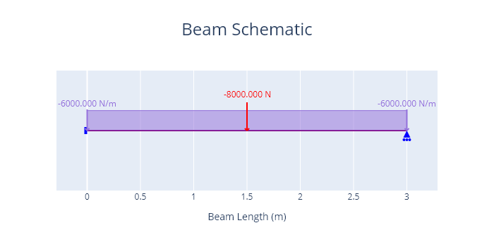
Specifications
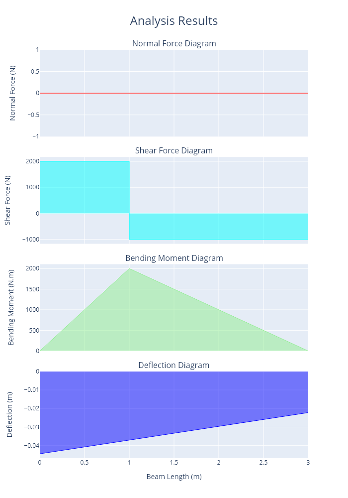
A 3 m long propped cantilever AB is fixed at A (x = 0 m), and supported on a roller at B (x = 3 m).
The beam is subject to a load of 8000 N acting downwards at the midspan, and a UDL of 6000 N/m across the length of the support.
E and I are constant.
A diagram of the problem is shown below.
Results
The following values can be directly extracted using the get_shear_force, get_bending_moment and get_reaction methods:
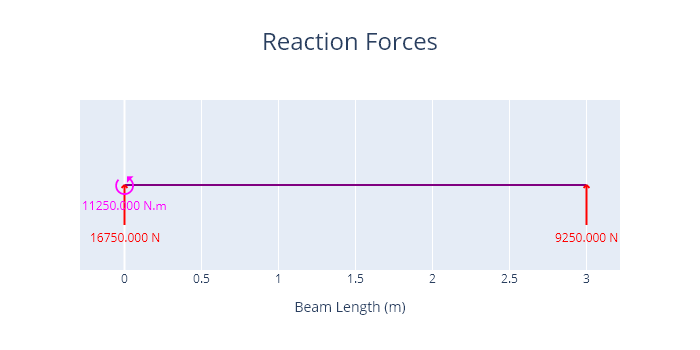
The absolute maximum shear force –> 16750 N
The absolute maximum bending moment –> 11250 N.m
The reaction at B –> 9250 N
A plot of the reactions is shown below.
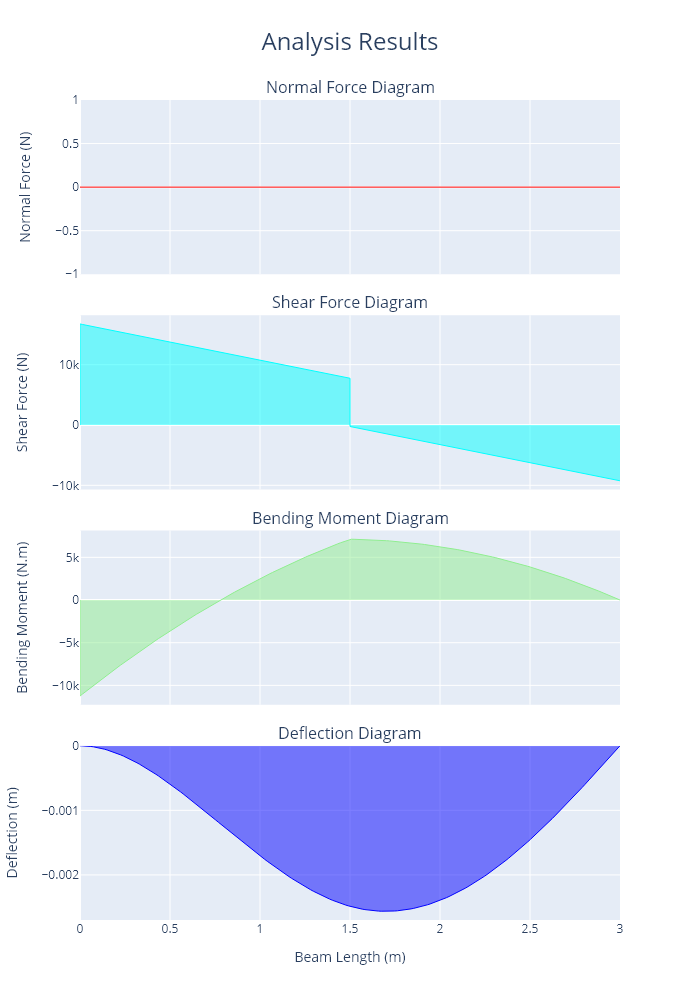
A plot of the axial force, shear force, and bending moments is shown below. A deflection graph is also presented however this depends on the beam properties E and I which werent included in this question. As a default the values E and I are taken as the values for a 150UB18.0 steel beam.
Code
# Statically Indeterminate beam (Ex 12.21 Hibbeler)
# Determine the reactions at the roller support B of the beam described below:
# 3 m long, fixed at A (x = 0 m), roller support at B (x=3 m),
# vertical point load at midpan of 8000 N, UDL of 6000 N/m, EI constant.

beam = Beam(3)

a = Support(0,(1,1,1))
b = Support(3,(0,1,0))

load_1 = PointLoadV(-8000,1.5)
load_2 = UDLV(-6000, (0,3))

beam.add_supports(a,b)
beam.add_loads(load_1,load_2)

beam.analyse()

print(f"The beam has an absolute maximum shear force of: {beam.get_shear_force(return_absmax=True)} N")
print(f"The beam has an absolute maximum bending moment of: {beam.get_bending_moment(return_absmax=True)} N.mm")
print(f"The beam has a vertical reaction at B of: {beam.get_reaction(3,'y')} N")

fig1 = beam.plot_beam_external()

fig2 = beam.plot_beam_internal()

fig1.update_layout(width=600)
fig2.update_layout(width=600)

fig_1.write_html("./example_1_external.html")
fig_2.write_html("./example_1_internal.html")
7. Spring Supported Beam
This example has been taken from Ex 12.16 in the Hibbeler textbook [2].
Specifications
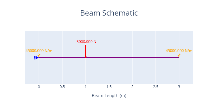
A 3 m long beam has spring supports at A (x = 0 m) and B (x = 3 m).
Both spring supports have a stiffness of 45 kN/m.
A downwards vertical point load of magnitude 3000 N acts at x = 1 m.
The beam has a Young’s Modulus (E) of 200 GPa and a second moment of area (I) of 4.6875*10**-6 m4.
Determine the vertical displacement at x = 1 m.
A diagram of the problem is shown below.
Results
The deflection is -0.0370370392 m
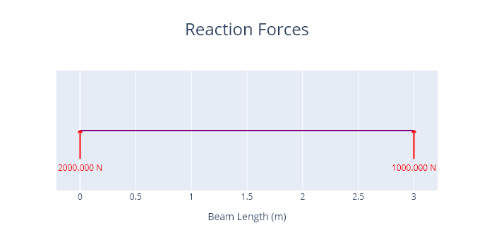
A plot of the reactions is shown below.
A plot of the axial force, shear force, and bending moments is shown below.
Code
# Spring Supported beam (Ex 12.16 Hibbeler)
# Determine the vertical displacement at x = 1 m for the beam detailed below:
# 3 m long, spring of ky = 45 kN/m at A (x = 0 m) and B (x = 3 m), vertical point load at x = 1 m of 3000 N, E = 200 GPa, I = 4.6875*10**-6 m4.

# when initializing beam we should specify E and I. Units should be expressed in MPa (N/mm2) for E, and mm4 for I
beam = Beam(3, E=(200)*10**3, I=(4.6875*10**-6)*10**12)

# creating supports, note that an x support must be specified even when there are no x forces. This will not affect the accuracy or reliability of results.
# Also note that ky units are kN/m in the problem but must be in N/m for the program to work correctly.
a = Support(0, (1,1,0), ky = 45000)
b = Support(3, (0,1,0), ky = 45000)

load_1 = PointLoadV(-3000, 1)

beam.add_supports(a,b)
beam.add_loads(load_1)

beam.analyse()

beam.get_deflection(1)

fig1 = beam.plot_beam_external()
fig1.show()

fig2 = beam.plot_beam_internal()
fig2.show()

##results in 38.46 mm deflection ~= 38.4mm specified in textbook (difference only due to their rounding)
##can easily check reliability of answer by looking at deflection at the spring supports. Should equal F/k.
## ie at support A (x = 0 m), the reaction force is 2kN by equilibrium, so our deflection is F/K = 2kn / 45*10-3 kN/mm = 44.4 mm (can be seen in plot)
8. Axially Loaded Indeterminate Beam
This example has been taken from Ex 4.13 in the Hibbeler textbook [2].
Specifications
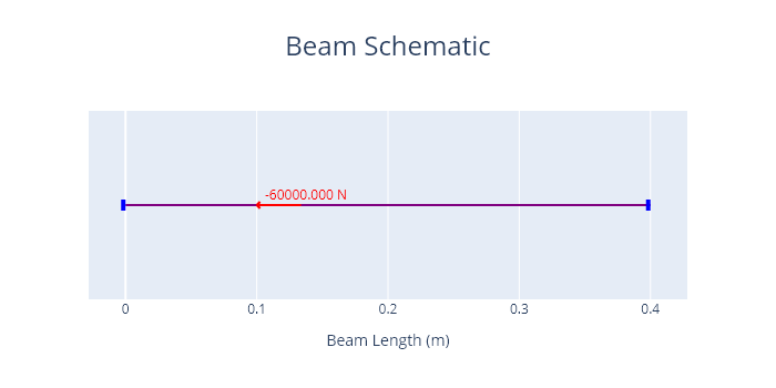
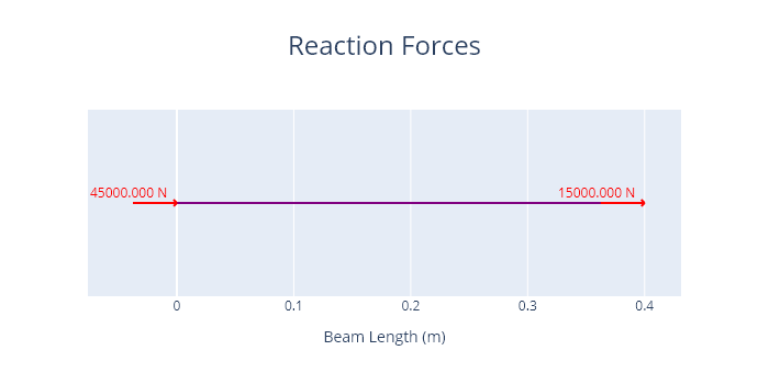
A rod with constant EA has a force of 60kN applied at x = 0.1 m, and the beam has fixed supports at x=0, and x =0.4 m. Determine the reaction forces.
A diagram of the problem is shown below.
Results
A plot of the reactions is shown below.
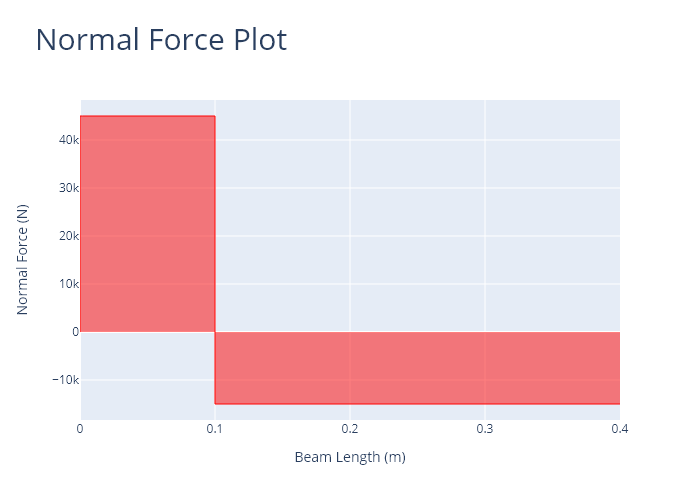
The normal force diagram is presented below.
Code
##AXIAL LOADED INDETERMINATE BEAM (Ex 4.13 Hibbeler)
## A rod with constant EA has a force of 60kN applied at x = 0.1 m, and the beam has fixed supports at x=0, and x =0.4 m. Determine the reaction forces.

beam = Beam(0.4)

a = Support()
b = Support(0.4)

load_1 = PointLoadH(-60000, 0.1)

beam.add_supports(a,b)
beam.add_loads(load_1)

beam.analyse()
beam.plot_normal_force()
9. Timoshenko Beam Theory
This example is a comparison of the Timoshenko beam theory and the Euler-Bernoulli beam theory for a multispan beam.
Specifications
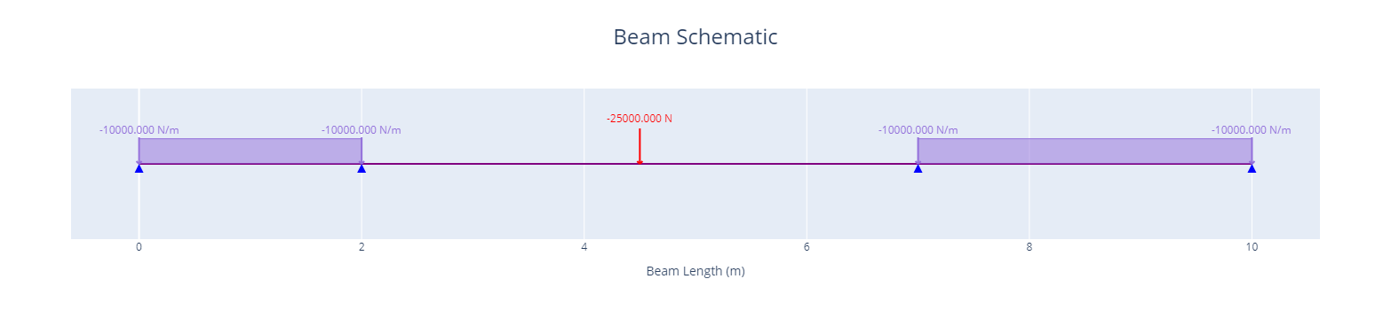
A beam is split up into a 2 m, 5 m and 3 m segment all pin supported. The outer spans have a 10 kN/m load and the middle span has a central point load of 25 kN. Show the deformations given the following section properties and compare to the Euler-Bernoulli beam theory:
E = 24.8 GPa
I = 11600 cm4
A = 74 cm2
G = 3.6 GPa
A diagram of the problem is shown below.
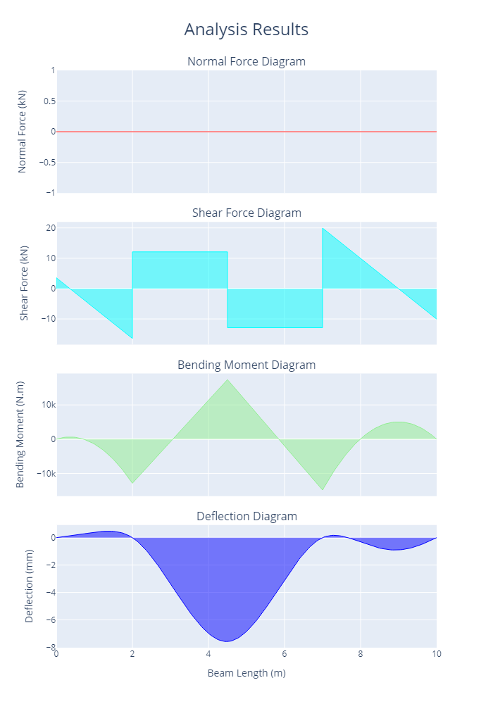
Results
The expected deflections using the SCIA software are as shown in the image below.
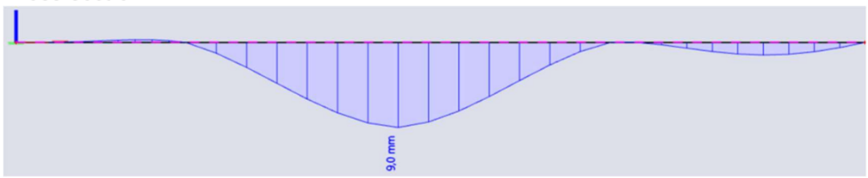
We observe that for timoshenko beam theory we get the same deflection as SCIA of 9mm. When using the Euler-Bernoulli beam theory we get a lower deflection of 7.6 mm and we can observe different reaction forces since the beam stiffness affects the distribution of forces in an indeterminate beam.
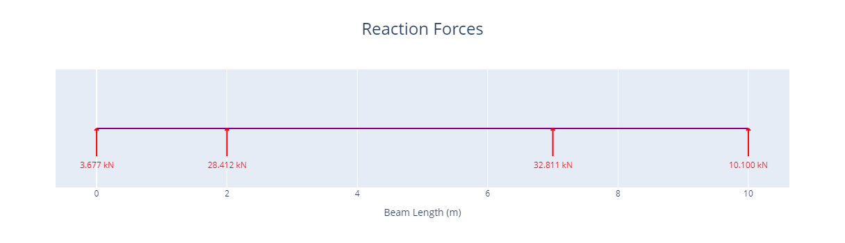
A plot of the reactions is shown below when using the Timoshenko beam theory.
A plot of the axial force, shear force, and bending moments is shown below using the Timoshenko beam theory.

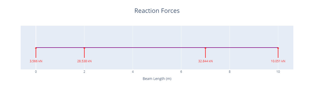
A plot of the reactions is shown below when using the Euler-Bernoulli beam theory.
A plot of the axial force, shear force, and bending moments is shown below using the Euler-Bernoulli beam theory.
Code
# TIMOSHENKO BEAM
beam = Beam(10, E=24800, G=3600, I=11600, A=74)

beam.update_units("E", "MPa")
beam.update_units("G", "MPa")
beam.update_units("I", "cm4")
beam.update_units("A", "cm2")
beam.update_units("force", "kN")
beam.update_units("distributed", "kN/m")
beam.update_units("deflection", "mm")

a = Support(0, (1, 1, 0))  # Defines a pin support at location x = 0 m
b = Support(2, (1, 1, 0))  # Defines a pin support at location x = 2 m
c = Support(7, (1, 1, 0))  # Defines a pin support at location x = 7 m
d = Support(10, (1, 1, 0))  # Defines a pin support at location x = 10 m

beam.add_supports(a, b, c, d)

load_1 = DistributedLoadV(-10, (0, 2))
load_2 = DistributedLoadV(-10, (7, 10))
load_3 = PointLoadV(-25, 4.5)
# Defines a point load of 1000 N acting up, at location x = 2 m
beam.add_loads(
    load_1, load_2, load_3
)  # Assign the support objects to a beam object created earlier

beam.analyse()

## plot the diagram of the problem
fig_0 = beam.plot_beam_diagram()
fig_0.show()

fig_1 = beam.plot_reaction_force()
fig_1.show()

fig_2 = beam.plot_beam_internal()
fig_2.show()

# EULER BEAM
beam = Beam(10, E=24800, I=11600, A=74)

beam.update_units("E", "MPa")
beam.update_units("I", "cm4")
beam.update_units("A", "cm2")
beam.update_units("force", "kN")
beam.update_units("distributed", "kN/m")
beam.update_units("deflection", "mm")

# assign supports and loads from earlier
beam.add_supports(a, b, c, d)
beam.add_loads(load_1, load_2, load_3)

beam.analyse()

## plot the results for the beam
fig_3 = beam.plot_reaction_force()
fig_3.show()

fig_4 = beam.plot_beam_internal()
fig_4.show()